 ARISE Home
 ARISE Data Center
Science
ARISE results
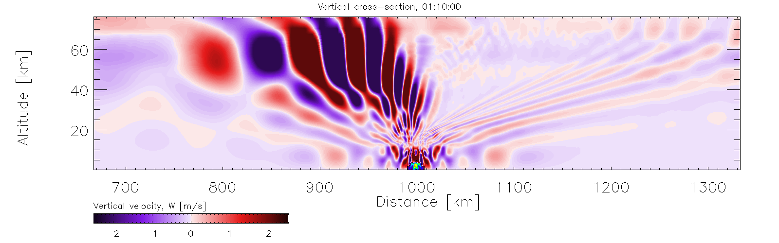
Numerical modelling of gravity wave propagation
Simulation by a regional meteorological model of gravity waves generated by a tropical thunderstorm. The figure shows the vertical cross section of the vertical velocity and the simulated thunderstorm.
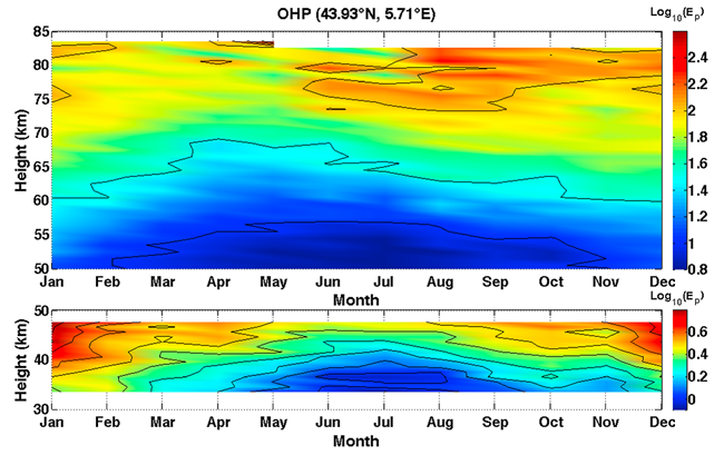
Gravity wave potential energy climatology from lidar observations
Observations of the Rayleigh lidar at OHP have been analyzed over a period of 16 years in order to build a climatology of GW potential energy at northern middle-latitudes. The above figure shows the contour plots of the gravity wave potential energy (Ep) climatology. As expected, we find an annual cycle with a maximum of gravity wave activity occurring in winter and a minimum in summer in the upper stratosphere (30–50 km). An annual cycle is also observed with maximum in winter and minimum during summer in the lower mesosphere (50–60 km). We found a semiannual cycle with maxima of gravity wave potential energy occurring in winter and in summer and minima occurring during the equinoxes in the upper mesosphere. A secondary maximum of the gravity wave activity occurs in summer (June, July, and August) at ~75 km. Looking at the seasonally averaged profiles, it is possible to observe the preferential altitudes of energy dissipation. Gravity waves are dissipating above ~70 km during all seasons, but there is relatively little dissipation at lower altitudes.
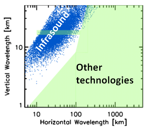
Gravity wave scales observed by the Ivory Coast infrasound station
Most gravity waves are too small to be explicitly resolved by general circulation models; instead parameterizations are used to simulate the drag on the mean flow caused by wave breaking. However, the paucity of measurements means that parameterization schemes are often tuned to produce more realistic temperature structures near the tropopause, or to improve representation of winds, rather than to replicate the actual deposition of gravity wave momentum. ARISE infrasound observations can be used to measure small scale gravity waves that are not observed by other techniques. The figure shows the typical horizontal and vertical scales measured by existing techniques (shown by the green shading, and gravity waves detected by the IS17 infrasound array (blue dots) in Ivory Coast, where the wave source is tropical convection. This improved resolution provides a long-term data set of gravity waves at parameterization scales.
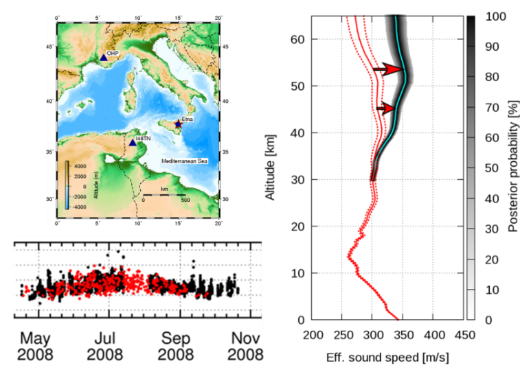
Observations of winds derived from infrasound
Accurate description of wind and temperature in the lower and middle atmosphere is needed by a wide variety of atmospheric sciences and applications, including the use of infrasound as a verification technique for the Comprehensive Nuclear-Test-Ban Treaty (CTBT) and Numerical Weather Prediction models. ARISE studies demonstrate the applicability of inverse problem to derive in higher spatial and temporal resolution the vertical structure of stratospheric wind and temperature using infrasound measurements from repetitive calibration sources. Thorough analyses of repetitive signals from Mt. Etna (Italy, 37.7°N, 15.0°E) recorded in the IMS Tunisian infrasound station, are used to evaluate the ECMWF model. Infrasound measurements following volcanic eruptions allow one to compare forecasted and real wind speeds. The red curve represents the a priori model and the black curve the inversion result. The dashed red lines indicate the intrinsic uncertainty in the model due to unresolved small-scale structure. The dark patched areas correspond to the a posteriori model distribution.
Assessment of operational network performance modelling
Validated numerical modelling techniques provide now a basis to better understand the role of different factors describing the source and the atmosphere that influence propagation predictions. In order to account for a realistic description of the dynamic structure of the atmosphere, model predictions are further enhanced by wind and temperature error distributions as measured in the framework of the first ARISE Design Study Project. The simulations below quantify uncertainties in the spatial and temporal variability of the detection thresholds of the IMS infrasound network.
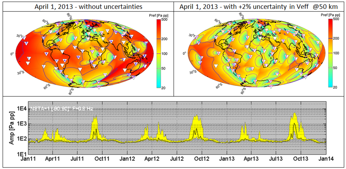
Effects of 2% uncertainties in the atmospheric model on the detection capability of the global IMS infrasound network. Simulations are carried out without (top left) and with (top right) incorporating ±2% uncertainties in the wind speed at 50 km altitude. The lower graph shows the median (black curve) and 95% confidence intervals (yellow region) of the global detection thresholds. The ARISE observation network will contributes to a better description of the stratospheric wind dynamics and related uncertainties, allowing reliable confidence levels to be associated with natural hazards notifications such like automatic notification of on-going volcanic eruption. In the context of the future verification of the CTBT, improved atmospheric models will be extremely helpful to assess the IMS network performance in higher resolution, to design and prioritize maintenance of any arbitrary infrasound monitoring network, and also improve source characterization methods used by a growing scientific community involved in operational infrasound monitoring.
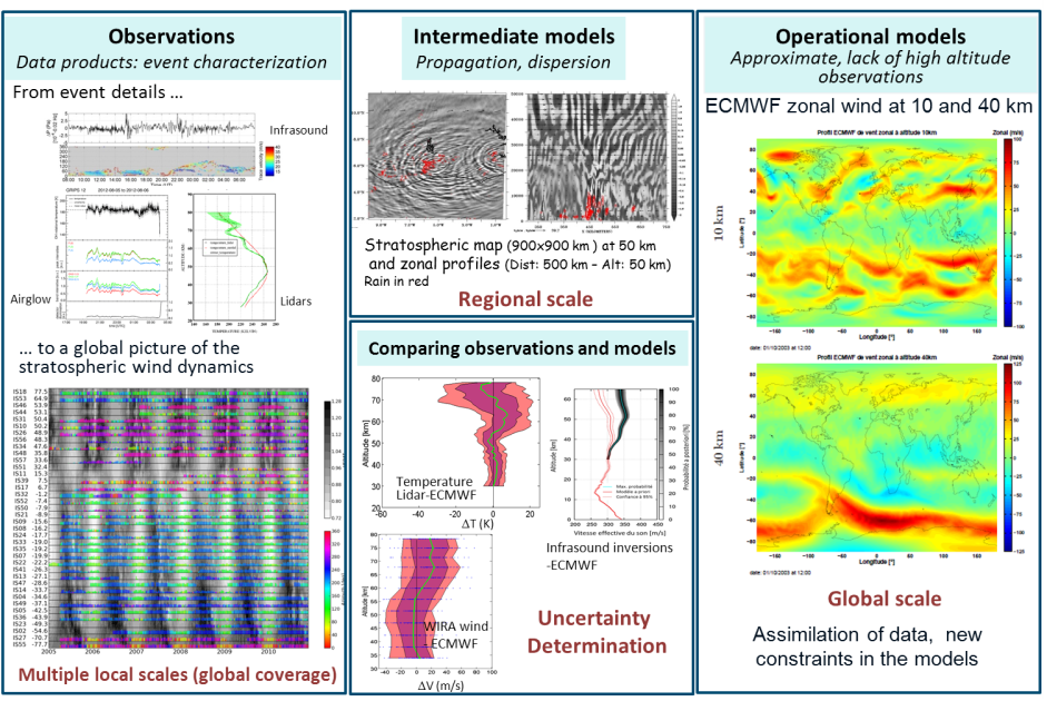
From observations to operational models
The aim of the ARISE project is to provide high resolution measurements in the SMLT (Stratosphere-Mesosphere-Lower Thermosphere) region which is currently sparsely sampled. The ultimate objective is to assimilate ARISE measurements by operational Numerical Weather Prediction centres to improve their estimate of the atmospheric state above 40 km. This would likely produce both a positive impact on NWP forecast skill and also provide additional constraint for some of the other data sources currently assimilated.
Comparison of co-located independent middle-atmosphere measurements with Numerical Weather Prediction models
High-resolution, ground-based and independent observations including wind radiometer, lidar and infrasound instruments are used to evaluate the accuracy of weather and climate models in the middle atmosphere at northern hemisphere mid-latitudes. Systematic comparisons between model output and observations are carried out in both time temporal and spectral domains on time scales ranging from one day to decades.
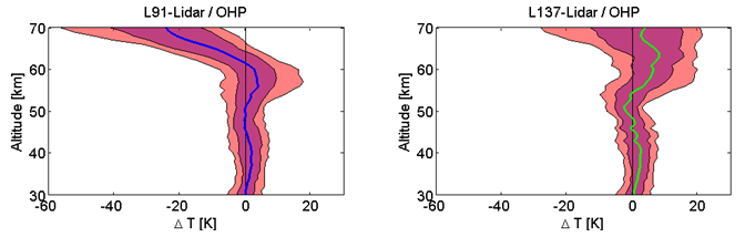
The figure presents the distribution of the differences between the ECMWF (European Centre for Medium-Range Weather Forecasts) temperature models and lidar observations during the OHP measurement campaign. On average, L91 and lidar are in good agreement up to the stratopause with a small positive difference of ~3 K. The median of the differences increases with altitude and reaches -35 K at 75 km. When using L137, differences are comparable to those below 50 km. However, above 60 km, the negative difference significantly reduces with a median of ±5 K and a 95% distribution of ±20 K.